实验报告
课程名称:计算机语音技术
实验题目:短时分析应用
学号:21281280
姓名:柯劲帆
班级:物联网2101班
指导老师:朱维彬
报告日期:2023年10月29日
---
# 目录
[TOC]
---
# 1. 短时能量和短时过零率函数
**添加短时时域参数函数:**
- **短时能量**
- **短时过零率**
## 1.1. 计算短时能量
短时能量指在语音信号的不同时间段内,信号的能量或振幅的平均值。
短时能量的计算公式如下:
$$
E_{n}=\sum_{m=-\infty}^{\infty}[x\left(m\right) h\left(n-m\right)]^{2}=\sum_{m=n-N+1}^{n}[x\left(m\right) h\left(n-m\right)]^{2}
$$
其中$h\left(n\right)$为窗函数,这里选择为海明窗:
$$
h\left(n\right)=\left\{\begin{array}{ll}
0.54 - 0.4\cos\left[2\pi n / \left(N - 1\right)\right], & 0 \leq n \leq N-1 \\
0, & \text { others }
\end{array}\right. \\
$$
因此使用Python定义计算海明窗的函数如下。(numpy库也有内置的海明窗函数,这里手动实现,和numpy的接口一致)
```python
def hamming(frame_length:int) -> np.ndarray:
# frame_length - 窗长
n = np.arange(frame_length)
h = 0.54 - 0.4 * np.cos(2 * np.pi * n / (frame_length - 1))
return h
```
**计算短时能量的算法:将每一帧的语音信号提取出来,乘上窗长并平方,然后求和取平均,即可得出该帧的短时能量。将窗口移动步长个单位,重复前面的流程,直至分析完整段语音。**
使用Python实现如下。
```python
def ampf(x: np.ndarray, FrameLen: Optional[int] = 128, inc: Optional[int] = 90) -> np.ndarray:
# x - 语音时域信号
# FrameLen - 每一帧的长度
# inc - 步长
frames = []
for i in range(0, len(x) - FrameLen, inc):
frame = x[i : i + FrameLen]
frames.append(frame)
frames = np.array(frames)
h = hamming(frame_length=FrameLen)[::-1] / FrameLen
amp = np.dot(frames ** 2, h.T ** 2).T
return amp
```
画出`tang1`的短时能量曲线如下:
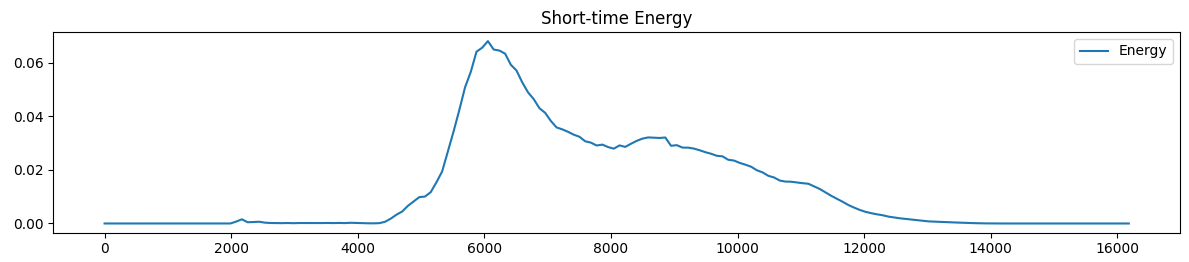
短时能量体现了该帧的振幅,可以表征韵母的发声和结束。
## 1.2. 计算短时过零率
短时过零率指在语音信号的短时段内,信号穿过水平线(即振幅为0)的次数。定义如下:
窗函数:
$$
w\left(n\right)=\left\{\begin{array}{ll}
\frac{1}{2 N}, & 0 \leq n \leq N-1 \\
0, & \text { others }
\end{array}\right. \\
$$
短时过零率:
$$
Z_{n}=\sum_{m=-\infty}^{\infty}\left|\operatorname{sgn}\left[x\left(m\right)\right]-\operatorname{sgn}\left[x\left(m-1\right)\right]\right| w\left(n-m\right)
$$
其中$\operatorname{sgn}$是符号函数:
$$
\operatorname{sgn}\left(x\left(n\right)\right)=\left\{\begin{array}{ll}
1, & x\left(n\right) \geq 0 \\
-1, & x\left(n\right)<0
\end{array}\right.
$$
**计算短时过零率的算法:先从语音信号中计算出过零序列(经过$\operatorname{sgn}$转化后,后一信号减前一信号)。然后将每一帧的语音信号对应的过零序列提取出来,求和并除以帧长,即为该帧的过零率。将窗口移动步长个单位,重复前面的流程,直至分析完整段语音。**
使用Python实现如下:
```python
def zcrf(x: np.ndarray, FrameLen: Optional[int] = 128, inc: Optional[int] = 90) -> np.ndarray:
# x - 语音时域信号
# FrameLen - 每一帧的长度
# inc - 步长
sound = x
sgn_sound = np.sign(sound)
dif_sound = np.abs(sgn_sound[1:] - sgn_sound[:-1])
frames = []
for i in range(0, len(dif_sound) - FrameLen, inc):
frame = dif_sound[i : i + FrameLen]
frames.append(frame)
frames = np.array(frames)
h = np.ones((FrameLen,)) / (2 * FrameLen)
zcr = np.dot(frames, h.T).T
return zcr
```
画出`tang1`的短时过零率曲线如下:
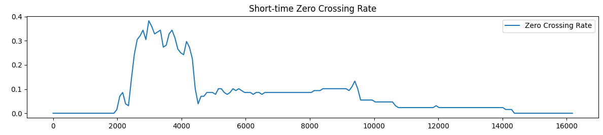
短时过零率体现了该帧的高频声音,可以表征声母的发声。
# 2. 边界检测
**添加边界检测器,基于短时能量、短时过零率,实现边界检测功能,包括**
- **语音端点检测——起始边界x1、终止边界x2**
- **清/浊边界检测x3**
我将每个发音分为3个阶段:
1. 未发声阶段:此时短时能量和短时过零率都很低
2. 声母阶段:此时声母的塞音、擦音和塞擦音等会产生大量的高频声波,过零率较大;但是此时韵母还没发出,短时能量较低。这一阶段的开始为`x1`。
3. 韵母阶段:此时韵母发出,频率趋于平稳和下降,因此此时过零率下降,但短时能量激增,并逐渐减少,直至发声完毕,回到1阶段。这一阶段的开始为`x3`,结束为`x2`。
**一开始将阶段初始化为`1`未发声阶段;接着当过零率高于阈值时,进入`2`声母阶段,添加`x1`;接着当短时能量高于阈值时,进入`3`声母阶段,添加`x3`;在进入`2`或`3`阶段后,当短时能量和短时过零率同时低于阈值时,重置为`1`未发声阶段,添加`x2`。**
**另外还设置了一个阈值宽度,当语音信号在大于阈值宽度的信号段满足条件才算通过。**
使用Python实现如下:
```python
sr, sound_array = wav.read(filename)
sound_array = sound_array.T[0, :] if sound_array.ndim != 1 else sound_array # 双通道改单通道
sound_array = sound_array / np.max(np.abs(sound_array)) # 归一化
amp = ampf(sound_array, FrameLen, inc)
zcr = zcrf_delta(sound_array, FrameLen, inc)
rescale_rate = len(sound_array) / amp.shape[0]
frameTime = np.arange(len(amp)) * rescale_rate
# 将曲线图拉伸至和语音信号图一样长,方便分析
x1 = []
x2 = []
x3 = []
amp2 = np.min(amp) + (np.max(amp) - np.min(amp)) * 0.05
zcr2 = np.min(zcr) + (np.max(zcr) - np.min(zcr)) * 0.04
threshold_len = 6
state = 1
for i in range(threshold_len, len(amp) - threshold_len):
if state == 1:
if np.all(zcr[i : i + threshold_len] > zcr2):
x1.append(i * rescale_rate)
state = 2
elif state == 2:
if np.all(amp[i : i + threshold_len] > amp2):
x3.append(i * rescale_rate)
state = 3
if state != 1 and np.all(amp[i : i + threshold_len] < amp2) and np.all(zcr[i : i + threshold_len] < zcr2):
x2.append(i * rescale_rate)
state = 1
```
阈值参数的选取在下一节中分析。
# 3. 绘制图像与分析
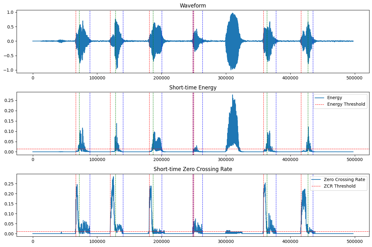
**绘制语音边界检测图,包括**
- **语音波形、短时能量、短时过零率**
- **自动检测结果:音段起始/终止边界、清音/浊音边界**
使用Python实现如下:
```python
# 绘制语音波形、短时能量、短时过零率
plt.figure(figsize=(12, 8))
# 语音波形
plt.subplot(3, 1, 1)
plt.plot(sound_array)
plt.title("Waveform")
for boundary in x1:
plt.axvline(x=boundary, color="r", linestyle="--", linewidth=0.8)
for boundary in x2:
plt.axvline(x=boundary, color="b", linestyle="--", linewidth=0.8)
for boundary in x3:
plt.axvline(x=boundary, color="g", linestyle="--", linewidth=0.8)
# 短时能量
plt.subplot(3, 1, 2)
plt.plot(frameTime, amp, label="Energy")
plt.axhline(y=amp2, color="r", linestyle="--", label="Energy Threshold", linewidth=0.8)
plt.legend()
plt.title("Short-time Energy")
for boundary in x1:
plt.axvline(x=boundary, color="r", linestyle="--", linewidth=0.8)
for boundary in x2:
plt.axvline(x=boundary, color="b", linestyle="--", linewidth=0.8)
for boundary in x3:
plt.axvline(x=boundary, color="g", linestyle="--", linewidth=0.8)
# 短时过零率
plt.subplot(3, 1, 3)
plt.plot(frameTime, zcr, label="Zero Crossing Rate")
plt.axhline(y=zcr2, color="r", linestyle="--", label="ZCR Threshold", linewidth=0.8)
plt.legend()
plt.title("Short-time Zero Crossing Rate")
for boundary in x1:
plt.axvline(x=boundary, color="r", linestyle="--", linewidth=0.8)
for boundary in x2:
plt.axvline(x=boundary, color="b", linestyle="--", linewidth=0.8)
for boundary in x3:
plt.axvline(x=boundary, color="g", linestyle="--", linewidth=0.8)
plt.tight_layout()
plt.show()
```
将`x1`语音开始边界标记为红色,`x2`语音结束边界标记为蓝色,将`x3`声韵母边界标记为绿色。
画出`tang1`的语音边界检测图如下:
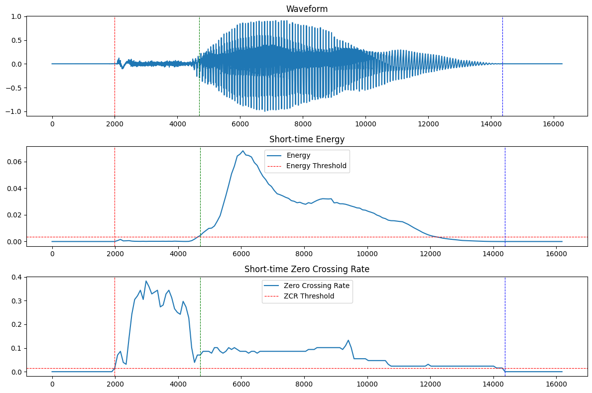
一共有3个参数:阈值宽度、短时能量阈值、短时过零率阈值
观察短时能量曲线和短时过零率曲线可见,声母开始时,短时能量曲线有一个小峰值,而短时过零率曲线出现大峰值,因此短时能量阈值必须高于该小峰值,才不会将声母开始判定为韵母开始。
韵母开始时,短时能量曲线出现大峰值,因此短时能量阈值应在大峰值和小峰值之间,且尽可能偏小,才能准确预测声韵母边界,经过多次实验,将短时能量阈值定为最大值的$5\%$;而短时过零率曲线回落,并在低值维持一段时间。因此短时过零率阈值要小于这个低值,经过多次实验,将短时过零率阈值定为最大值的$4\%$。
经过多次实验,将阈值宽度定为$6$帧。
从检测结果来看,上述参数的选择能够较为准确地区分三个边界。但是声韵母边界有少许滞后于真实边界。
# 4. 自录制语音检测、分析与算法优化
自录制一段语音:“计算机语音技术”,检测与绘图如下:
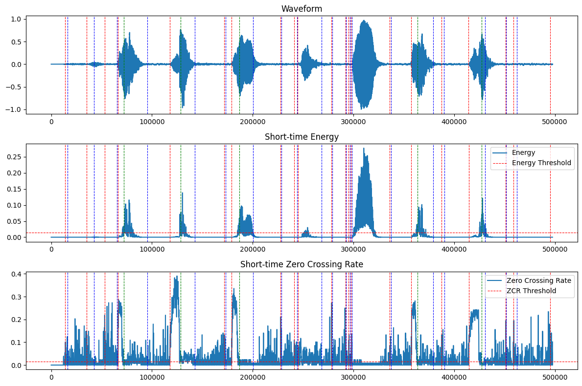
很显然,噪声较大,严重干扰了分析。
分析可知,噪声主要影响的是短时过零率。因此,我对短时过零率算法进行了优化,采用了噪声背景下的修正$\operatorname{sgn}$函数:
$$
\operatorname{sgn}\left(x\left(n\right)\right)=\left\{\begin{array}{ll}
1, & x\left(n\right) \geq \Delta \\
-1, & x\left(n\right)< -\Delta\\
0, & \text{others}
\end{array}\right.
$$
在具体的实现中,我使用矩阵运算语音信号,逐采样点判断$x\left(n\right)$和$\pm \Delta$的大小既不经济,也不优雅。因此,我首先将$x\left(n\right)$进行了变换,即将修正$\operatorname{sgn}$函数改写为:
$$
\operatorname{sgn}\left(x\left(n\right)\right)=\left\{\begin{array}{ll}
1, & x\left(n\right) \geq 0 \wedge x\left(n\right) - \Delta \geq 0\\
-1, & x\left(n\right) < 0 \wedge x\left(n\right) + \Delta< 0\\
0, & \text{others}
\end{array}\right.
$$
相当于正负值信号都向横坐标轴缩减了$\Delta$,再进行普通的$\operatorname{sgn}$操作。
所以,首先将语音信号减去阈值$\Delta$,去掉负值信号,得到正值信号;将语音信号加上阈值$\Delta$,去掉正值信号,得到负值信号。再将两者相加合并,得到处理后的语音信号。最后,进行普通的普通的$\operatorname{sgn}$函数操作。
Python实现如下:
```python
def delta_sgn(x: np.ndarray) -> np.ndarray:
# x - 语音信号
sound = x
threshold = np.max(np.abs(sound)) * 0.05
negative_sound = sound + threshold
negative_sound -= np.abs(negative_sound)
positive_sound = sound - threshold
positive_sound += np.abs(positive_sound)
sound = (negative_sound + positive_sound) / 2
sound = np.sign(sound)
return sound
```
画出向横坐标轴缩减了$\Delta$的语音信号(下)与原语音信号(上)的对比图:
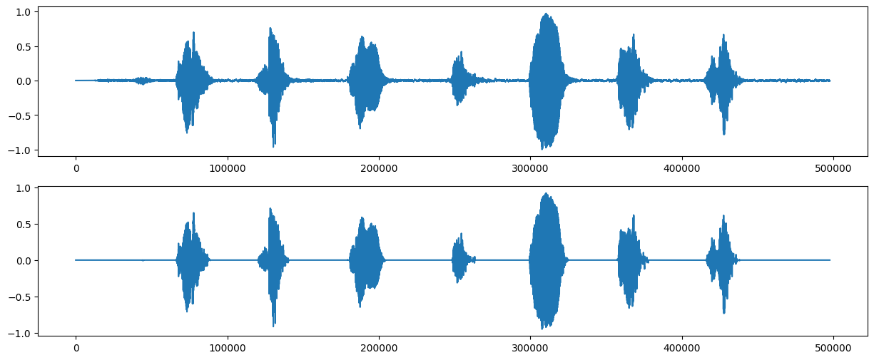
很明显,噪声几乎被消除了。
接下来使用上面定义的`delta_sign()`函数,重复之前的计算进行分析和画图:
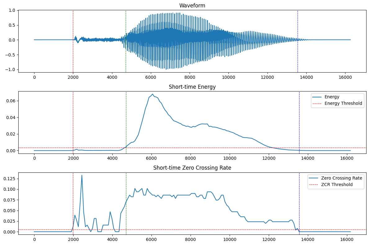
可以看到,算法能够在噪声下辨认出`ji4`、`suan4`、`ji1`、`ji4`和`shu4`这4个发音的发声起止边界和声韵母边界,但是`yu3`和`yin1`两个发音没有声母,在仅用短时能量和短时过零率两个指标的条件下无法正常检测出边界。另外由于算法抑制了一部分噪声,韵母发音的最后一小部分被消除了,因此检测到的发音结束边界较正确的结束边界有所提前。
将改进后的算法应用到`tang1`的音频中,检测结果如下:
发现其声母`t`阻塞阶段的高频声音被抑制了,但由于音量较大,没有被作为噪声消除,依然能被正常识别。但是发音末尾的少部分被当作噪声消除了,导致发音结束边界较正确的结束边界有所提前。检测结果总体上正确。