实验报告
课程名称:计算机语音技术
实验题目:实验3
学号:21281280
姓名:柯劲帆
班级:物联网2101班
指导老师:朱维彬
报告日期:2023年10月13日
---
[TOC]
---
# 1. 自相关系数计算和基音周期候选点集
- **基于自相关系数AC的局部极大值构成基音周期候选点集,通过预设基频范围进行初步筛选**
## 1.1. 计算自相关系数
自相关算法能够体现语音信号的时域重复性。
基于某帧语音信号的自相关函数的在某一时延$t$(单位为采样点)的大小,可以推断该帧语音信号的基音周期是$t$的可能性:$t$点自相关系数越大,基音周期是$t$的概率越大;反之亦然。
因此,可以通过计算语音信号中各帧的自相关函数来推断各帧的基音周期。
自相关函数的计算方法:
$$
\hat{R}_n\left(k\right) = \sum_{m=0}^{N-1}x\left(n+m\right)x\left(n+m+k\right)
$$
其中$\hat{R}_n\left(k\right)$是第$k$帧的自相关函数,其中$0\le k < N$,$N$为语音的分帧数。
代码实现如下:
```python
# 读取音频文件
filename = "./tang1.wav"
sample_rate, sound_array = scipy.io.wavfile.read(filename)
sound_array = sound_array.T[0, :] if sound_array.ndim != 1 else sound_array
sound_array = sound_array / np.max(np.abs(sound_array)) # 归一化
frame_length = int(sample_rate * 0.01)
num_frames = len(sound_array) // frame_length
autocorrelation = np.zeros((num_frames, frame_length)) # 每帧的自相关函数
autocorrelation_of_candidates = np.zeros((num_frames, frame_length))
for n in range(num_frames):
frame = sound_array[n * frame_length: (n + 1) * frame_length] # 提取单帧
autocorrelation[n, :] = scipy.signal.correlate(frame, frame, mode='full')[frame_length - 1:]
```
代码的逻辑为:
1. 读取音频文件并进行预处理;
2. 设置帧长和分帧数,以及初始化自相关函数的记录变量;
3. 逐帧进行自相关计算。
## 1.2. 选取基音周期候选点集
得到自相关函数`autocorrelation`后,下一步就是取各帧的局部极大值构成基音周期候选点集。
但是在实际实验中,局部极大值的提取较为困难:要么就是自相关函数波动严重,局部极大值非常多;要么就是自相关函数单调变化或平滑变化,局部极大值几乎不存在。由于后续的DP算法需要每一帧都有基音周期候选点集,所以局部极大值数量少会严重影响算法的稳定性。
因此,考虑到一帧的长度不大,我**将符合人声基频范围的所有基音周期都视为候选点**。那么基音周期候选点的范围限制为:
$$
\frac{1}{min\times \frac{1}{sample \space rate}} \le 80\rm{Hz}\Longrightarrow min \ge \frac{sample \space rate}{80\rm{Hz}}
$$
同理,
$$
\frac{1}{max\times \frac{1}{sample \space rate}} \ge 400\rm{Hz}\Longrightarrow max \le \frac{sample \space rate}{400\rm{Hz}}
$$
综上,基音周期候选点的范围为
$$
\left [\frac{sample \space rate}{400\rm{Hz}}, \frac{sample \space rate}{80\rm{Hz}}\right ]
$$
为了让DP算法只选择在阈值内的基音周期(即不选择阈值外的基音周期),所以将阈值外的自相关系数置为一个较小的数,从而让DP算法选择阈值外基音周期的代价变高。
代码实现如下:
```python
min_peak_threshold = min(sample_rate // 400, frame_length)
max_peak_threshold = min(sample_rate // 80, frame_length)
autocorrelation_of_candidates = autocorrelation
autocorrelation_of_candidates[:, 0:min_peak_threshold] = np.min(autocorrelation) - 5.
autocorrelation_of_candidates[:, max_peak_threshold:] = np.min(autocorrelation) - 5.
```
最终,`tang1.wav`的自相关函数计算结果如下所示,
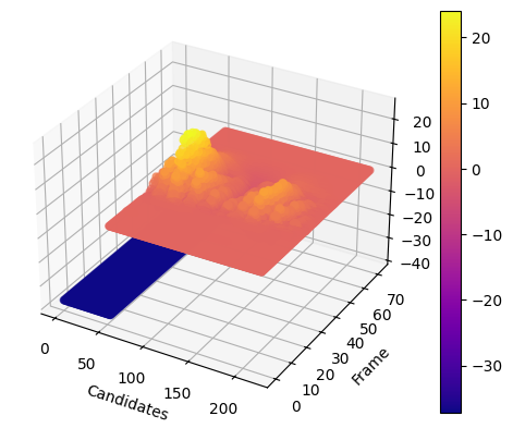 $x$轴为帧,$y$轴为候选点,$z$轴为自相关函数。不在人声基频范围内的点的自相关系数被置为一个很低的数值(蓝色区域所示)。
# 2. 动态规划DP算法
- **采用动态规划DP算法,通过代价函数`CostFunction() `涉及目标、转移代价,利用帧同步搜索代价最小路径,检测出基频**
DP算法的步骤如下:
1. **初始化第$1$帧的代价函数**
$$
CostF\left(1, i\right) = Dist\left(ac\left({Can}_{1}\left(i\right)\right)\right) \left ( i=1, 2, \dots, L \right )
$$
其中:
- $CostF\left(n, i\right)$表示第$n$帧的第$i$个基音周期候选点的累计代价;
- $Dist\left(\right)$为距离测度;
- $ac\left(\right)$表示自相关函数序列;
- ${Can}_{n}\left(i\right)$表示第$n$帧的第$i$个基音周期候选点;
- $L$表示候选点数。
我将$Dist\left(\right)$的计算设置为
$$
Dist\left(ac\left({Can}_{1}\left(i\right)\right)\right) = - \operatorname{normalize} \left(ac\left({Can}_{1}\left(i\right)\right)\right) \times 2 \times10^6
$$
其中$\operatorname{normalize} \left(\right)$表示归一化,这是为了控制不同的音频计算得到的不同自相关系数在固定的范围。
代码实现如下:
```python
costF = np.zeros((num_frames, frame_length))
path = np.zeros((num_frames, frame_length))
dist = -(autocorrelation_of_candidates - np.min(autocorrelation_of_candidates)) / (np.max(autocorrelation_of_candidates) - np.min(autocorrelation_of_candidates)) * 2e3
costF[0, :] = dist[0, :]
```
代码声明了代价记录变量和转移路径记录变量,然后初始化第$1$帧的代价函数。
2. **计算每帧的代价函数**
$$
\begin{array}{c}
CostF\left(n+1, j\right) = \underset{i}{\operatorname{min}}\left(CostF\left(n, i\right)+CostT\left(n, i, j\right)\right)+CostG\left(n+1, j\right)\\
Path = \underset{i}{\operatorname{argmin}}\left(CostF\left(n, i\right)+CostT\left(n, i, j\right)\right)\left ( i,j=1, 2, \dots, L \right )
\end{array}
$$
其中:
- $CostT\left(n, i, j\right)$表示转移代价:第$n$帧中第$i$个候选点的基频与第$n+1$帧中第$j$个候选点的基频之差,并进行归一化;
- $CostG\left(n+1, j\right)$为目标代价:等于$Dist\left(ac\left({Can}_{n+1}\left(j\right)\right)\right)$的值。
这一步是要计算得到的结果满足两个评价指标的权衡:
- 自相关系数尽可能大,即基音周期正确概率尽可能大;
- 基频的变化尽可能小,即基音周期的变化尽可能小。
这两个指标都进行了归一化操作,即都在$\left[0, 1\right]$之间,只需要调整它们的权重即可人工控制权衡的决策。这里,我将自相关系数相关的权重设置为$2 \times10^6$,基音周期变化的权重设置为$1$。
代码实现如下:
```python
for n in range(num_frames - 1):
for j in range(min_peak_threshold, max_peak_threshold):
costT = np.abs(sample_rate / np.arange(frame_length)[1:] - sample_rate / j)
costT = (costT - np.min(costT)) / (np.max(costT) - np.min(costT))
costG = dist[n + 1, j]
costF[n + 1, j] = costG + np.min(costF[n, 1:] + costT)
path[n + 1, j] = np.argmin(costF[n, 1:] + costT) + 1
```
代码循环计算了每帧的代价函数。
3. **确定最优路径**
$$
\hat{l}_N=\underset{j}{\operatorname{argmin}}\left(CostF\left(N, j\right)\right)
$$
即找到累计代价最小的结束帧作为预测结果的结束帧。
代码实现如下:
```python
l_hat = np.zeros(num_frames, dtype=np.int32)
l_hat[num_frames - 1] = np.argmin(costF[num_frames - 1, 1:]) + 1
```
4. **路径回溯**
$$
\begin{array}{c}
\hat{l}_n=Path\left(n+1, \hat{l}_{n+1}\right)\\
F0\left [ n \right ] = F0\left ( {Can}_{n}\left(\hat{l}_n\right) \right )
\end{array}
$$
即从后一帧往前推出使得代价最小的前一帧(代价最小的转移路径已经在`Path`变量中记录),然后计算出该帧的基频。
由候选点计算基频的公式为:
$$
F0\left ({Can}_{n}\left(i\right) \right ) = \frac{sample \space rate}{{Can}_{n}\left(i\right)}
$$
代码实现如下:
```python
for n in range(num_frames - 2, -1, -1):
l_hat[n] = path[n + 1, l_hat[n + 1]]
f0 = sample_rate / l_hat
```
运行以上代码,并画出语音信号及基频变化如下:
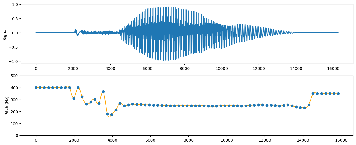
使用Praat进行基频检测,预测基频如下:
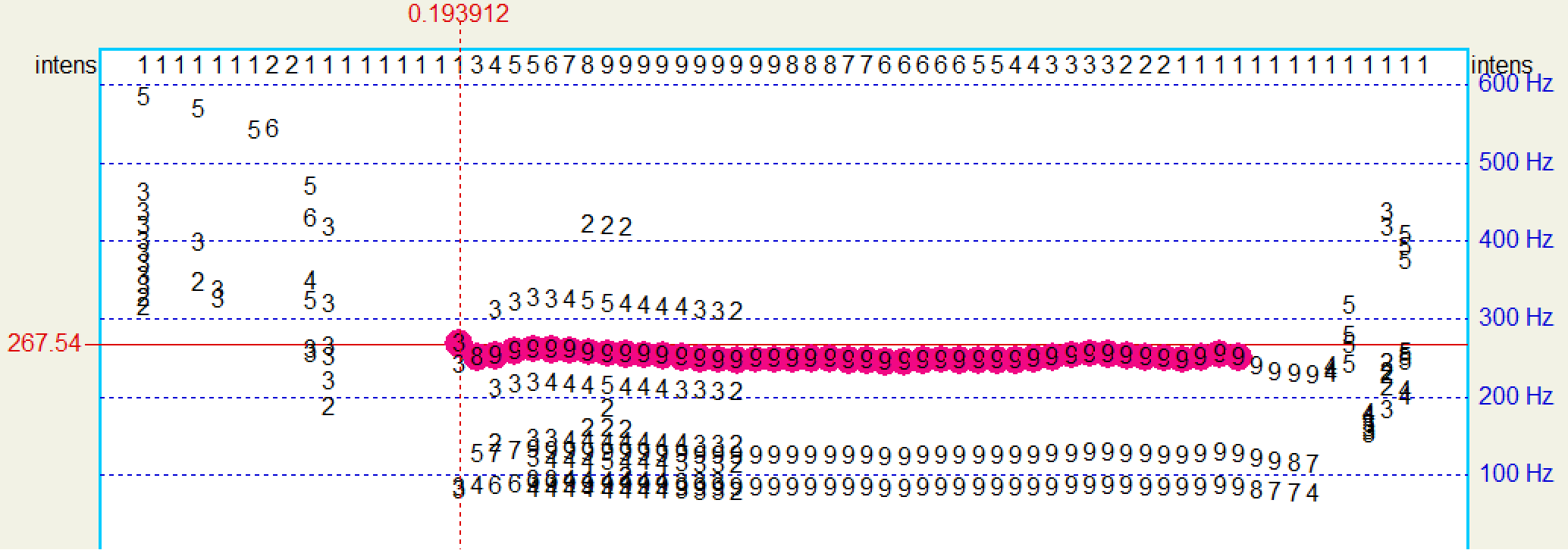
预测结果相近,表明算法基本正确。
# 3. 绘制图像与分析
- **自行录制一段连续语音发音,对检测结果进行分析,针对观察到的问题优化算法**
使用实验1中录制的“wo3 jiao4 ke1 jing4 fan1”作为测试音频,进行基频分析。
自相关函数如下:
$x$轴为帧,$y$轴为候选点,$z$轴为自相关函数。不在人声基频范围内的点的自相关系数被置为一个很低的数值(蓝色区域所示)。
# 2. 动态规划DP算法
- **采用动态规划DP算法,通过代价函数`CostFunction() `涉及目标、转移代价,利用帧同步搜索代价最小路径,检测出基频**
DP算法的步骤如下:
1. **初始化第$1$帧的代价函数**
$$
CostF\left(1, i\right) = Dist\left(ac\left({Can}_{1}\left(i\right)\right)\right) \left ( i=1, 2, \dots, L \right )
$$
其中:
- $CostF\left(n, i\right)$表示第$n$帧的第$i$个基音周期候选点的累计代价;
- $Dist\left(\right)$为距离测度;
- $ac\left(\right)$表示自相关函数序列;
- ${Can}_{n}\left(i\right)$表示第$n$帧的第$i$个基音周期候选点;
- $L$表示候选点数。
我将$Dist\left(\right)$的计算设置为
$$
Dist\left(ac\left({Can}_{1}\left(i\right)\right)\right) = - \operatorname{normalize} \left(ac\left({Can}_{1}\left(i\right)\right)\right) \times 2 \times10^6
$$
其中$\operatorname{normalize} \left(\right)$表示归一化,这是为了控制不同的音频计算得到的不同自相关系数在固定的范围。
代码实现如下:
```python
costF = np.zeros((num_frames, frame_length))
path = np.zeros((num_frames, frame_length))
dist = -(autocorrelation_of_candidates - np.min(autocorrelation_of_candidates)) / (np.max(autocorrelation_of_candidates) - np.min(autocorrelation_of_candidates)) * 2e3
costF[0, :] = dist[0, :]
```
代码声明了代价记录变量和转移路径记录变量,然后初始化第$1$帧的代价函数。
2. **计算每帧的代价函数**
$$
\begin{array}{c}
CostF\left(n+1, j\right) = \underset{i}{\operatorname{min}}\left(CostF\left(n, i\right)+CostT\left(n, i, j\right)\right)+CostG\left(n+1, j\right)\\
Path = \underset{i}{\operatorname{argmin}}\left(CostF\left(n, i\right)+CostT\left(n, i, j\right)\right)\left ( i,j=1, 2, \dots, L \right )
\end{array}
$$
其中:
- $CostT\left(n, i, j\right)$表示转移代价:第$n$帧中第$i$个候选点的基频与第$n+1$帧中第$j$个候选点的基频之差,并进行归一化;
- $CostG\left(n+1, j\right)$为目标代价:等于$Dist\left(ac\left({Can}_{n+1}\left(j\right)\right)\right)$的值。
这一步是要计算得到的结果满足两个评价指标的权衡:
- 自相关系数尽可能大,即基音周期正确概率尽可能大;
- 基频的变化尽可能小,即基音周期的变化尽可能小。
这两个指标都进行了归一化操作,即都在$\left[0, 1\right]$之间,只需要调整它们的权重即可人工控制权衡的决策。这里,我将自相关系数相关的权重设置为$2 \times10^6$,基音周期变化的权重设置为$1$。
代码实现如下:
```python
for n in range(num_frames - 1):
for j in range(min_peak_threshold, max_peak_threshold):
costT = np.abs(sample_rate / np.arange(frame_length)[1:] - sample_rate / j)
costT = (costT - np.min(costT)) / (np.max(costT) - np.min(costT))
costG = dist[n + 1, j]
costF[n + 1, j] = costG + np.min(costF[n, 1:] + costT)
path[n + 1, j] = np.argmin(costF[n, 1:] + costT) + 1
```
代码循环计算了每帧的代价函数。
3. **确定最优路径**
$$
\hat{l}_N=\underset{j}{\operatorname{argmin}}\left(CostF\left(N, j\right)\right)
$$
即找到累计代价最小的结束帧作为预测结果的结束帧。
代码实现如下:
```python
l_hat = np.zeros(num_frames, dtype=np.int32)
l_hat[num_frames - 1] = np.argmin(costF[num_frames - 1, 1:]) + 1
```
4. **路径回溯**
$$
\begin{array}{c}
\hat{l}_n=Path\left(n+1, \hat{l}_{n+1}\right)\\
F0\left [ n \right ] = F0\left ( {Can}_{n}\left(\hat{l}_n\right) \right )
\end{array}
$$
即从后一帧往前推出使得代价最小的前一帧(代价最小的转移路径已经在`Path`变量中记录),然后计算出该帧的基频。
由候选点计算基频的公式为:
$$
F0\left ({Can}_{n}\left(i\right) \right ) = \frac{sample \space rate}{{Can}_{n}\left(i\right)}
$$
代码实现如下:
```python
for n in range(num_frames - 2, -1, -1):
l_hat[n] = path[n + 1, l_hat[n + 1]]
f0 = sample_rate / l_hat
```
运行以上代码,并画出语音信号及基频变化如下:

使用Praat进行基频检测,预测基频如下:

预测结果相近,表明算法基本正确。
# 3. 绘制图像与分析
- **自行录制一段连续语音发音,对检测结果进行分析,针对观察到的问题优化算法**
使用实验1中录制的“wo3 jiao4 ke1 jing4 fan1”作为测试音频,进行基频分析。
自相关函数如下:
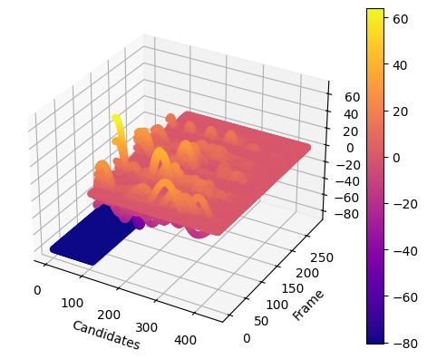 发现自相关函数比单音节的`tang1`的更加复杂,但是可以明显发现五个发音之间由四个空隙隔开——在这四个空隙中,自相关函数值相对较低,印证了发音间隙基频变化大的事实。
使用过DP算法计算后,画出基频曲线:
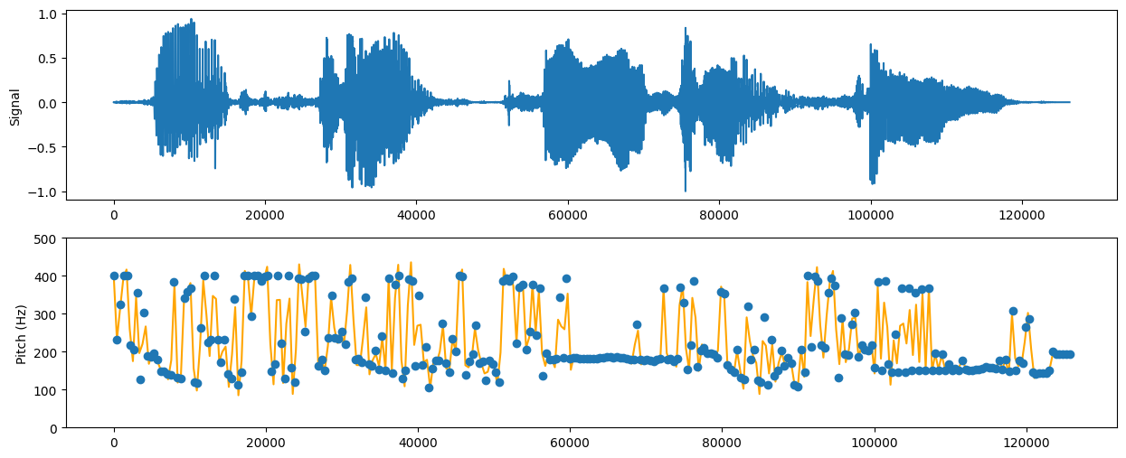
虽然可以大致判断基频变化情况,但是不明显。分析发现,基频变化太大了,因此需要调整转移代价的权重,增加基频转移对DP算法决策的惩罚。
因此,将
```python
dist = -autocorrelation_of_candidates * 2e3
```
修改为
```python
dist = -autocorrelation_of_candidates * 1e1
```
其余不变。再次运行并绘图:
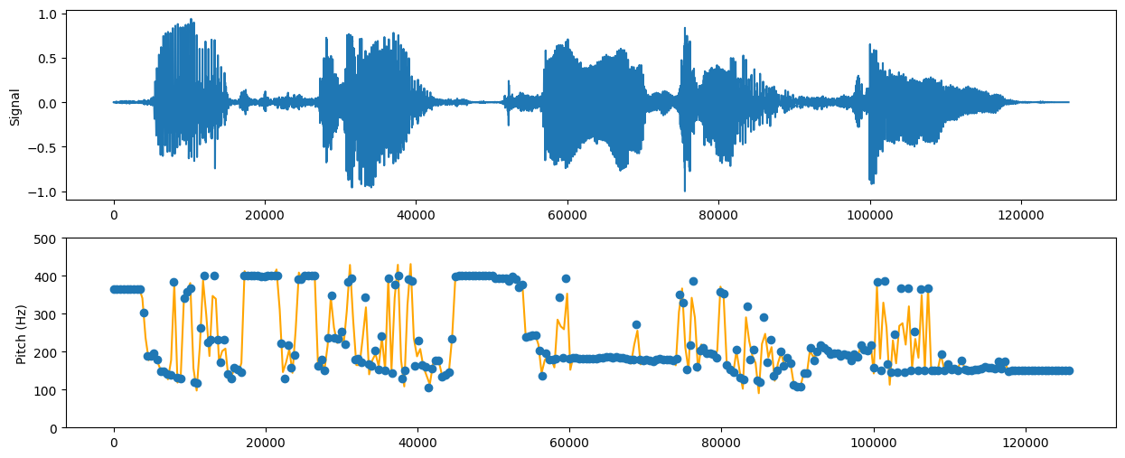
此时,基频更加集中,变化趋势较为明显。
与Praat的检测结果进行比对:
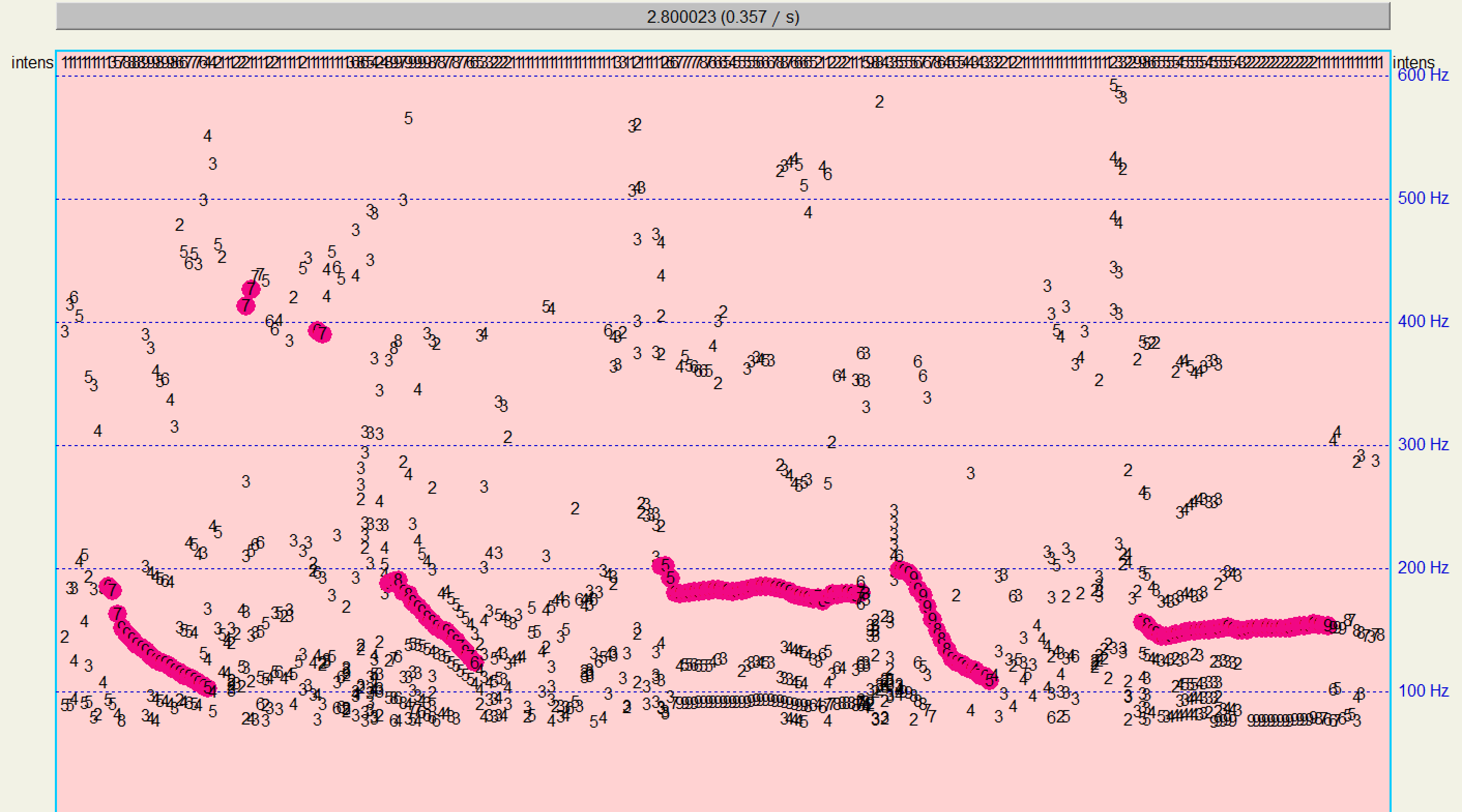
有较高的相似性,说明算法有效。
对于算法的优化调整,我只想到调整目标代价和转移代价两者之间的平衡权重进行优化。这个优化方法只能靠手动且经验性较强,效果不佳。
# 4. 附录
完整算法及绘图代码:
```python
import scipy
import numpy as np
import matplotlib.pyplot as plt
# 读取音频文件
filename = "./tang1.wav"
sample_rate, sound_array = scipy.io.wavfile.read(filename)
sound_array = sound_array.T[0, :] if sound_array.ndim != 1 else sound_array
sound_array = sound_array / np.max(np.abs(sound_array)) # 归一化
frame_length = int(sample_rate * 0.01)
num_frames = len(sound_array) // frame_length
autocorrelation = np.zeros((num_frames, frame_length))
autocorrelation_of_candidates = np.zeros((num_frames, frame_length))
# 基频阈值为80-400Hz,则基音周期(即延迟)t最小为sample_rate/400,最大为sample_rate/80
min_peak_threshold = min(sample_rate // 400, frame_length)
max_peak_threshold = min(sample_rate // 80, frame_length)
for n in range(num_frames):
frame = sound_array[n * frame_length: (n + 1) * frame_length]
autocorrelation[n, :] = scipy.signal.correlate(frame, frame, mode='full')[frame_length - 1:]
# 本应该使用峰值的延迟作为基音周期的候选值,但是发现峰值(局部极大值)并不好判断,同时一帧内的点数不多,因此将阈值内的所有点都作为候选点
# 那么将不在阈值内的自相关系数置为一个非常小的数,从而不让算法选择不在阈值内的基音周期
autocorrelation_of_candidates = autocorrelation
autocorrelation_of_candidates[:, 0:min_peak_threshold] = np.min(autocorrelation) - 10.
autocorrelation_of_candidates[:, max_peak_threshold:] = np.min(autocorrelation) - 10.
x, y = np.meshgrid(np.arange(frame_length), np.arange(num_frames))
x, y, z = x.flatten(), y.flatten(), autocorrelation_of_candidates.flatten()
fig = plt.figure()
ac_3d = fig.add_subplot(111, projection='3d')
sc = ac_3d.scatter(x, y, z, c=z, cmap='plasma')
ac_3d.set_xlabel('Candidates')
ac_3d.set_ylabel('Frame')
ac_3d.set_zlabel('AC Value')
plt.colorbar(sc)
plt.show()
costF = np.zeros((num_frames, frame_length))
path = np.zeros((num_frames, frame_length))
dist = -(autocorrelation_of_candidates - np.min(autocorrelation_of_candidates)) / (np.max(autocorrelation_of_candidates) - np.min(autocorrelation_of_candidates)) * 1e1
costF[0, :] = dist[0, :]
for n in range(num_frames - 1):
for j in range(min_peak_threshold, max_peak_threshold):
# f0 = sample_rate / candidate
costT = np.abs(sample_rate / np.arange(frame_length)[1:] - sample_rate / j)
costT = (costT - np.min(costT)) / (np.max(costT) - np.min(costT)) # 归一化
costG = dist[n + 1, j]
costF[n + 1, j] = costG + np.min(costF[n, 1:] + costT)
path[n + 1, j] = np.argmin(costF[n, 1:] + costT) + 1
l_hat = np.zeros(num_frames, dtype=np.int32)
l_hat[num_frames - 1] = np.argmin(costF[num_frames - 1, 1:]) + 1
for n in range(num_frames - 2, -1, -1):
l_hat[n] = path[n + 1, l_hat[n + 1]]
f0 = sample_rate / l_hat
plt.figure(figsize=(15, 6))
plt.subplot(2, 1, 1)
plt.plot(sound_array)
plt.ylabel("Signal")
plt.subplot(2, 1, 2)
plt.ylim(0, 500)
x = frame_length * np.arange(num_frames)
y = f0
X_Smooth = np.linspace(x.min(), x.max(), 300)
Y_Smooth = scipy.interpolate.make_interp_spline(x, y)(X_Smooth)
plt.plot(X_Smooth, Y_Smooth, color="orange")
plt.plot(x, y, "o")
plt.ylabel("Pitch (Hz)")
plt.show()
```
发现自相关函数比单音节的`tang1`的更加复杂,但是可以明显发现五个发音之间由四个空隙隔开——在这四个空隙中,自相关函数值相对较低,印证了发音间隙基频变化大的事实。
使用过DP算法计算后,画出基频曲线:

虽然可以大致判断基频变化情况,但是不明显。分析发现,基频变化太大了,因此需要调整转移代价的权重,增加基频转移对DP算法决策的惩罚。
因此,将
```python
dist = -autocorrelation_of_candidates * 2e3
```
修改为
```python
dist = -autocorrelation_of_candidates * 1e1
```
其余不变。再次运行并绘图:

此时,基频更加集中,变化趋势较为明显。
与Praat的检测结果进行比对:

有较高的相似性,说明算法有效。
对于算法的优化调整,我只想到调整目标代价和转移代价两者之间的平衡权重进行优化。这个优化方法只能靠手动且经验性较强,效果不佳。
# 4. 附录
完整算法及绘图代码:
```python
import scipy
import numpy as np
import matplotlib.pyplot as plt
# 读取音频文件
filename = "./tang1.wav"
sample_rate, sound_array = scipy.io.wavfile.read(filename)
sound_array = sound_array.T[0, :] if sound_array.ndim != 1 else sound_array
sound_array = sound_array / np.max(np.abs(sound_array)) # 归一化
frame_length = int(sample_rate * 0.01)
num_frames = len(sound_array) // frame_length
autocorrelation = np.zeros((num_frames, frame_length))
autocorrelation_of_candidates = np.zeros((num_frames, frame_length))
# 基频阈值为80-400Hz,则基音周期(即延迟)t最小为sample_rate/400,最大为sample_rate/80
min_peak_threshold = min(sample_rate // 400, frame_length)
max_peak_threshold = min(sample_rate // 80, frame_length)
for n in range(num_frames):
frame = sound_array[n * frame_length: (n + 1) * frame_length]
autocorrelation[n, :] = scipy.signal.correlate(frame, frame, mode='full')[frame_length - 1:]
# 本应该使用峰值的延迟作为基音周期的候选值,但是发现峰值(局部极大值)并不好判断,同时一帧内的点数不多,因此将阈值内的所有点都作为候选点
# 那么将不在阈值内的自相关系数置为一个非常小的数,从而不让算法选择不在阈值内的基音周期
autocorrelation_of_candidates = autocorrelation
autocorrelation_of_candidates[:, 0:min_peak_threshold] = np.min(autocorrelation) - 10.
autocorrelation_of_candidates[:, max_peak_threshold:] = np.min(autocorrelation) - 10.
x, y = np.meshgrid(np.arange(frame_length), np.arange(num_frames))
x, y, z = x.flatten(), y.flatten(), autocorrelation_of_candidates.flatten()
fig = plt.figure()
ac_3d = fig.add_subplot(111, projection='3d')
sc = ac_3d.scatter(x, y, z, c=z, cmap='plasma')
ac_3d.set_xlabel('Candidates')
ac_3d.set_ylabel('Frame')
ac_3d.set_zlabel('AC Value')
plt.colorbar(sc)
plt.show()
costF = np.zeros((num_frames, frame_length))
path = np.zeros((num_frames, frame_length))
dist = -(autocorrelation_of_candidates - np.min(autocorrelation_of_candidates)) / (np.max(autocorrelation_of_candidates) - np.min(autocorrelation_of_candidates)) * 1e1
costF[0, :] = dist[0, :]
for n in range(num_frames - 1):
for j in range(min_peak_threshold, max_peak_threshold):
# f0 = sample_rate / candidate
costT = np.abs(sample_rate / np.arange(frame_length)[1:] - sample_rate / j)
costT = (costT - np.min(costT)) / (np.max(costT) - np.min(costT)) # 归一化
costG = dist[n + 1, j]
costF[n + 1, j] = costG + np.min(costF[n, 1:] + costT)
path[n + 1, j] = np.argmin(costF[n, 1:] + costT) + 1
l_hat = np.zeros(num_frames, dtype=np.int32)
l_hat[num_frames - 1] = np.argmin(costF[num_frames - 1, 1:]) + 1
for n in range(num_frames - 2, -1, -1):
l_hat[n] = path[n + 1, l_hat[n + 1]]
f0 = sample_rate / l_hat
plt.figure(figsize=(15, 6))
plt.subplot(2, 1, 1)
plt.plot(sound_array)
plt.ylabel("Signal")
plt.subplot(2, 1, 2)
plt.ylim(0, 500)
x = frame_length * np.arange(num_frames)
y = f0
X_Smooth = np.linspace(x.min(), x.max(), 300)
Y_Smooth = scipy.interpolate.make_interp_spline(x, y)(X_Smooth)
plt.plot(X_Smooth, Y_Smooth, color="orange")
plt.plot(x, y, "o")
plt.ylabel("Pitch (Hz)")
plt.show()
```